The Rabbit Hole Started With $P = \tau\,\omega$
Cycling is one of those rare sports where the input can be measured almost directly. The crank doesn’t care about vibes, power is power:
$$
P(t) = \tau(t)\,\omega(t)
$$
When I bought my first road bike, I tried to estimate power the hard way: stopwatch timing between traffic lights, a hand-wavy drag estimate, and some back-of-the-envelope aero. It was surprisingly close on flat roads… until I bought the “real” sensors: GPS, heart rate, and eventually a power meter.
Suddenly I had the kind of data stream my inner nerd can’t ignore: speed, elevation, slope, cadence, heart rate, and power all synchronized.
And of course that immediately turned into a coding project.
This project started years ago as a Perl script (I know…), and has gradually evolved into a more mature set of Python scripts.
If you want to poke around the code, it lives in this GitHub Repo
The current goal is simple to describe but tricky to do well:
Take a time history of measured power and predict the heart-rate response with a small, physically-motivated model and then fit the model parameters to real rides.
The Data: Five Channels That Tell the Whole Story
A typical ride provides multiple coupled signals: speed changes alter aerodynamic load, grade changes alter gravitational work, cadence shifts alter how you deliver power, and heart rate reacts with both delay and drift.
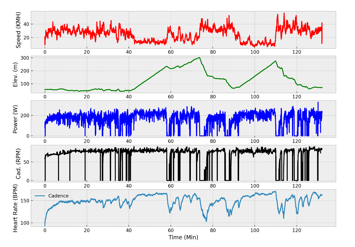 Typical ride time histories: speed, elevation, power, cadence, and heart rate.
A Heart-Rate Model as an ODE
At the core is a first-order dynamic system: heart rate evolves continuously in time in response to current power output and accumulated “stress.”
$$
\frac{d\,HR}{dt}
=
F\!\left(
P(t),\, P_{\max},\, P_{\text{low}},\, \tau_{\text{decay}},\, n,\,
HR_{\max},\, HR_{\text{low}},\, S(t)
\right)
$$
Where:
- $HR(t)$ is heart rate (BPM)
- $P(t)$ is measured power (W)
- $P_{\max},\,P_{\text{low}}$ anchor power capability
- $HR_{\max},\,HR_{\text{low}}$ bound physiological response
- $\tau_{\text{decay}}$ sets recovery time
- $n$ governs nonlinear fatigue accumulation
- $S(t)$ is an accumulated stress state
Stress as a Filtered Power Integral
The stress variable evolves as an integral of power:
$$
S(t) = \int_{0}^{t} \left(\frac{P(t)-P_{\text{low}}}{P_{max}-P_{\text{low}}}\right)^n dt
$$
The heart rate then relaxes toward a power- and stress-dependent target:
$$
\frac{dHR}{dt}
=
\frac{1}{\tau_{HR}}
\left(
HR_{\text{target}}(P,S) - HR
\right)
$$
Parameter Fitting as an Optimization Problem
Given a ride with $N$ samples, the model is simulated forward using the measured power input. The parameters $\theta$ are chosen to minimize mismatch with measured heart rate.
$$
\theta =
\left[
P_{\max},\, P_{\text{low}},\, \tau_{\text{decay}},\, n,\,
HR_{\max},\, HR_{\text{low}}, \ldots
\right]
$$
Weighted RMS Objective
$$
J(\theta)
=
\sqrt{
\frac{1}{N}
\sum_{i=1}^{N}
w(HR_{\text{meas},i})
\left(
HR_{\text{model},i}(\theta)
-
HR_{\text{meas},i}
\right)^2
}
$$
Where the weight emphasizes accuracy at high heart rates:
$$
w(HR)
=
1
+
\alpha
\left(
\frac{HR - HR_{\text{low}}}
{HR_{\max} - HR_{\text{low}}}
\right)^p
$$
So now I have a model of how my own heart rate responds to the power I’m trying to generate with my legs.
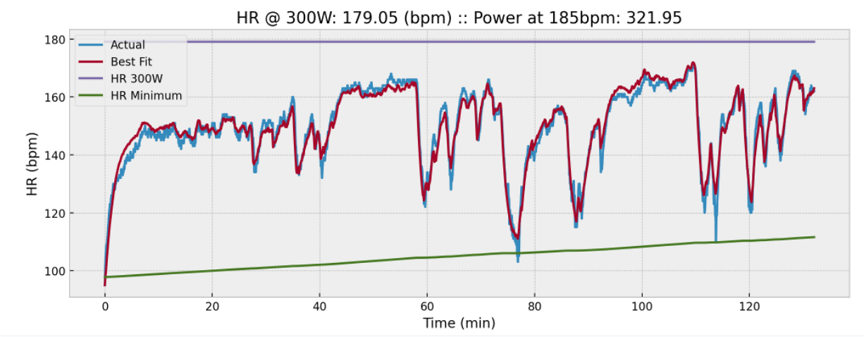 Fitted Heart Rate model versus data from my heart rate monitor
Optimization: Making It Fast and Robust
My first attempt used a hand-rolled gradient method. It worked, but it was slow and sometimes brittle.
Two changes made this practical:
- Renormalizing parameters to comparable numerical scales
- Switching to Nelder–Mead via SciPy
The result: a two-hour ride (~7200 samples) fits in about 30 seconds, down from ~10 minutes, with much better robustness.
What the Model Enables
Once fitted, the model lets me:
- Track fitness changes over time
- Observe reduced heart-rate drift for the same stress load
- Compare rides in a way that’s not tied to any single metric
And it unlocks the next step.
With:
- a fitted HR–power model,
- GPS elevation data,
- a physics-based bike model,
- and a rule-based pacing strategy,
I can simulate an entire course and predict speed, power, and heart rate histories.
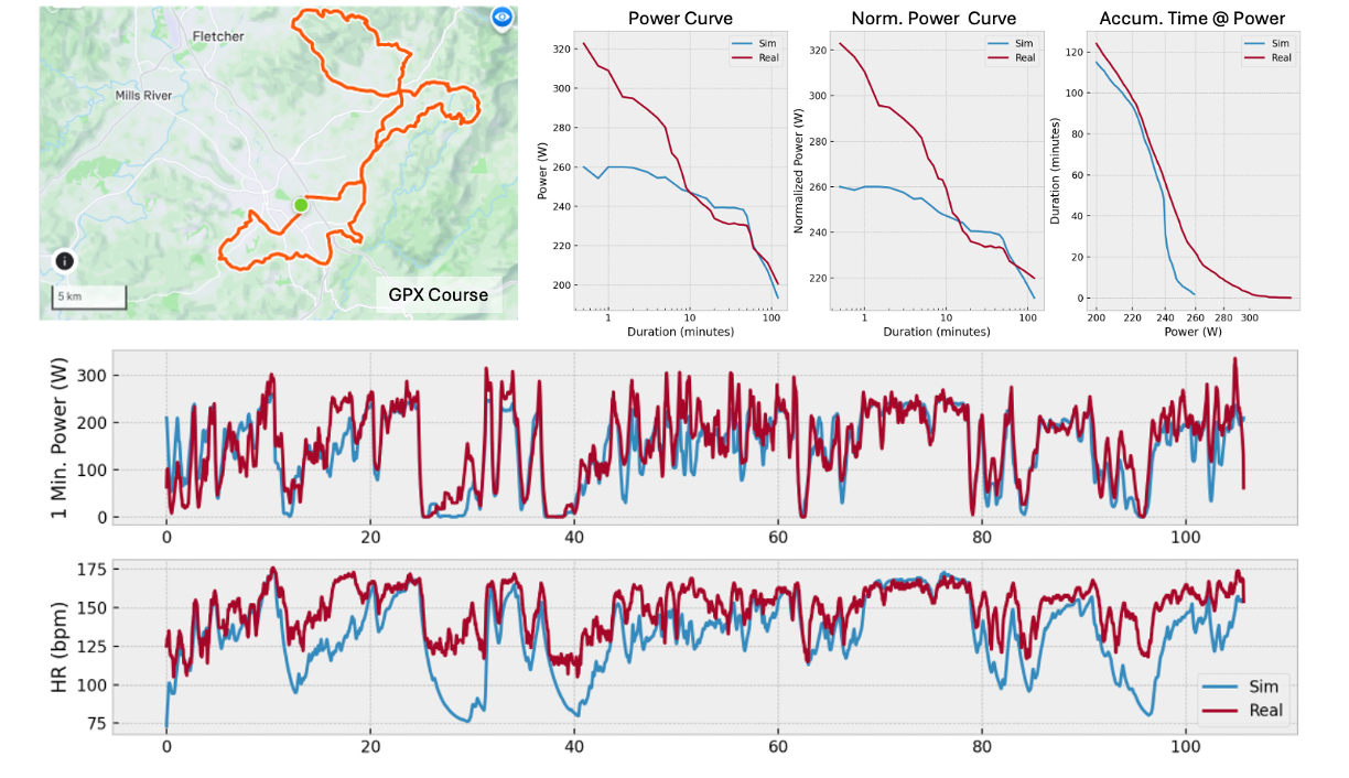 Measured versus simulated race performance.
The Next Step: Optimizing Pacing
Ultimately, this becomes an optimal control problem:
$$
\min_{P(t)} \; T
\quad
\text{s.t.}
\quad
\dot{HR} = f(HR,P,S),\;
\dot{S} = g(S,P),\;
HR \le HR_{\max},\;
0 \le P \le P_{\max}
$$
Choosing when to spend power is often more important than how much power you have.
Closing Thought
This project started with a single equation and grew into a modeling and optimization framework that blends physics, physiology, and numerical methods.
It’s also a reminder of why I love engineering: once intuition becomes a model, it becomes something you can test, refine, and reuse.
Ryan Blanchard PhD
Design, Research, Engineering, Data, Physics. I believe that few things in life are as rewarding as commiting yourself to a project to get something built. The feeling of seeing numerical and statistical models come to life in real-world hardware is just unbeatable.